Special relativity and the rod/slot paradox – XIX – perception of transit and collision scenario in a common reference frame

We continue our analysis of the so called “rod/slot paradox” in the Special Theory of Relativity. In this post we want to directly compare two important scenarios for possible rod/slot encounters – namely a collision scenario and a transit scenario – in a common reference frame. In contrast to the 17th post, we now pick our standard setup frame A, in which we defined a clear collision scenario, for our comparison (see the first posts of this series).

A transit scenario is one, which allows for a passage of the rod through the slot. We have already shown that a natural setup frame W for the definition of a clear and obvious transit scenario is a frame which moves diagonally in the setup frame A for the collision scenario. In such a frame W the rod moves horizontally and is passed by a vertically approaching slot. This corresponds to the logical and physical opposite of the collision scenario in A, in which the slot moves horizontally and the rod in vertical direction. The words “horizontal” and “vertical” in both cases refer to coordinate systems with x-axes parallel to the slot’s orientation there.

In the preceding posts, we have already performed a Lorentz Transformation [LT] of all relevant rod/slot data from frame W to frame A. We are now going to interpret the transformed data. Afterward we compare our scenarios side by side in frame A.

Previous posts ( a complete list is given at the end of the first post):

Motivation: The idea behind a direct comparison in one and the same reference frame is to demonstrate that the standard presentation of the rod/slot paradox does not at all compare these types of different scenarios, but instead ignores the impact of the the Thomas-Wigner rotation on the perception of both scenarios by different observers. A collision encounter remains a collision encounter in all frames of reference – and its conditions are profoundly different from those of a transit scenario – and vice versa.

Results of the preceding post

Let us call the rod and slot in the collision scenario “c-rod” and “c-slot“, and in the transit scenario “t-rod” and “t-slot“, respectively. For the setup of the positions and velocities of c-rod and the c-slot in the collision scenario see post II. For the basic setup of a transit scenario see post VIII – and for a corresponding setup in a diagonally moving frame W the preceding post XVII. I use the same notation for quantities as in the preceding post.

Note: For our comparison we have equipped the c-slot and t-slot with equal properties in W. We have given both slots the same length L (i.e. their proper lengths) and the same vertical velocity. We therefore expect that a Lorentz Transformation to frame A will reproduce equal properties of the slots there, too.

In the last two posts, I have thoroughly discussed how we link up our frames W and A in a reasonable way by a relative motion of their origins vs. each other. I have also discussed what this implies for a natural choice of the velocities of the t-rod and the t-slot in frame W. While all other velocities were fixed by the relative movement of W vs. A, we explicitly coupled the horizontal velocity of the t-rod in W to the relative velocity between the frames.

In this post we discuss the results of a LT for our reasonably chosen values of the velocity components in W. Our specific velocity settings makes the mathematical handling a bit easier – and it allows for the direct comparison of the scenarios in frame A. With our specific settings, the “transit scenario” is then perceived in frame A as displayed in the schematic drawing below:

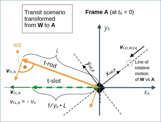
Perception of the transit scenario in frame A at t=0

Illustration 1: Schematic representation of the transit scenario in our standard frame A at t_A = 0. The drawing is based on the results of a Lorentz Transformation of the data for the t-rod and t-slot from a diagonally approaching natural setup frame W, which defines a clear and obvious transit scenario in a simple way. We have taken into account a specific, but natural choice of the horizontal velocity of the t-rod in W.

Readers who have followed this post series recognize the axes x_rel,A and y_rel,A of a rotated coordinate system, which has its x_rel,A -axis aligned with the line of relative motion of the frames versus each other. The rotated coordinate system was used to perform the Lorentz Transformation (in its simple form) from W to A.

A noteworthy side effect of our choice of the t-rod’s velocity in W is the following:

The t-rod gets the same length L as the c-rod in frame A. This makes a later comparison of the collision scenario with the transit scenario in A very instructive. We have equivalent slots and two rods of the same length there!

The diagonal movement of the t-rod to the left may appear a bit strange at first sight, because we set up the rod’s movement in W to the right along the chosen x_sW -axis there (see the last two posts). But the opposite direction in A along the x_A-axis is, of course, caused by the relative motion of W vs. A along a diagonal path down to the left in A – with velocity

\[ ||\pmb{v}_{rel,W2A} ||\,=\, v_{rel}\,. \]

For v_rel see below and/or previous posts. It is defined by the velocities of the c-rod and c-slot in A.

Properties of the t-slot in frame A

The Lorentz Transformation revealed that the t-slot resides on the x_A-axis in A and moves for t_A > 0 to the left with the same velocity (-ν_x) as the c-slot in the collision scenario. Its length L_ts,A is given by

\[ L_{ts,A} \,=\, {1 \over \gamma_x}\, L \,. \]

L is the proper length of both the rods and the slots at rest. At t_A = 0, the right end of the slot (x_ts,l,A) coincides with A’s origin, the related y-value is zero at this point in time:

\[ \begin{align} t_A = 0: \quad x_{ts,l, A} \,&=\, 0\,, \quad x_{ts,r, A} \,=\, L_{ts,A}\,, \\[8pt] y_{ts,r, A} \,&=\, 0\,, \quad y_{ts,r, A} \,=\, 0\,. \end{align} \]

The velocity components v_ts,x,A in x_A– and v_ts,y,A in y_A -direction are;

\[ t_A = 0: \quad v_{ts,x, A} \,=\, – \, \nu_x \,, \quad v_{ts,y, A} \,=\, 0\,. \]

ν_x is the absolute value of the horizontal velocity of the c-slot in the collision scenario in negative x_A– direction (with corresponding standard relativistic factors β_x and γ_x). ν_y is the absolute value of the vertical velocity of the c-rod in the collision scenario in negative y_A-direction (with corresponding standard relativistic factors β_y and γ_y). Remember that we have

\[ \begin{align} v_{rel} \,&=\, \left[\, \nu_x^2 \,+\, v_y^2 \,\right]^{1/2}\, \, \lt \, c\,, \\[8pt] \beta_{rel}^2 \,&=\, \beta_x^2 \,+\, \beta_y^2\, \, \lt \, 1 \,. \end{align}\]

The inequalities taking care of the relativistic limit c for the relative velocity.

Properties of the t-rod in frame A

It is a bit more difficult to describe the t-rod and its movement in A. Its length L_tr,A in frame A was found to assume a (maximum) value of L, due to our velocity settings:

\[ L_{tr,A} \,=\, L \,. \]

The angle inclination angle relative to the x_rel,_A-axis is given by

\[ \begin{align} \cos \left( \Psi_{tr,rel,A} \right) \,& =\, -\, {1 \over \gamma_{rel}} * {\beta_x \, \gamma_x \over \beta_{rel} \, \gamma_{rel}} \, {1 \over N^{1/2} } \,, \\[8pt] \sin \left( \Psi_{tr,rel,A} \right) \,& =\, +\, \gamma_x \, {\beta_y \over \beta_{rel}} \, {1 \over N^{1/2} } \,, \end{align} \]

with

\[ N \,=\, 1 \,-\, \beta_x^2 \, { \gamma_x^2 \over \, \gamma_{rel}^2} \,\lt\, 1 \,. \]

As we know that the cosine and sine of the angle Ψ_rel,A between the x_rel,_A -axis and the x_A-axis are

\[ |\cos \left( \Psi_{rel,A} \right) | \,=\, { \beta_x \over \beta_{rel} }\,, \quad |\sin \left( \Psi_{rel,A} \right) | \,=\, { \beta_y \over \beta_{rel} } \,, \]

we can, with a bit of trigonometry, derive formulas for the angle Ψ_tr,xA between the t-rod and the x_A-axis:

\[ \begin{align} \cos \left( \Psi_{tr,xA} \right) \,& =\, -\, {1 \over \gamma_x} \, {1 \over N^{1/2} } \,, \\[8pt] \sin \left( \Psi_{tr,xA} \right) \,& =\, +\, \gamma_x \, \beta_x \, \beta_y \, {1 \over N^{1/2} } \,. \end{align} \]

It is relatively easy to prove that these expressions give values which always are smaller than 1. I leave this small exercise to the reader. Another interesting quantity, which we later need, is the tangent of Ψ_tr,xA:

\[ \tan\left( \Psi_{tr,x,A} \right) \,=\, \gamma_x^2 \, \beta_x\, \beta_x \,. \]

Let us turn to the velocity vector v_tr,A of the t-rod. The norm of the vector v_tr,A has a value of

\[ v_{tr,A} \,=\, ||\pmb{v}_{tr,A}|| \,=\, \gamma_x \, {1 \over N^{1/2}} \, \beta_y * c \,. \]

Because the vector v_tr,A is perpendicular to the t-trod, the components v_tr,x,A and v_tr,y,A of v_tr,A parallel to the x_A-axis and the y_A-axis, respectively, are:

\[ \begin{align} v_{tr,x,A} \,&= \, – \, v_{tr,A} * |\sin \left( \Psi_{tr,xA} \right) | \\[8pt] &=\, – \, c \, {1\over N} \, \gamma_x^2 \, \beta_x \, \beta_y^2 \,, \\[10pt] v_{tr,y,A} \,&= \, – \, v_{tr,A} * |\cos \left( \Psi_{tr,xA} \right) | \\[8pt] &=\, – \, c \, {1\over N} \, \beta_y \,. \end{align} \]

A further evaluation of v_tr,x,A gives us

\[ v_{tr,x,A} \, = \, – \, (\beta_x * c) \, {\beta_y^2 \over \left[\, 1 \,-\, \beta_x^2 \,\right]^2 \,+\, \beta_x^2\, \beta_y^2} \,. \]

Using the relativistic limit condition for v_rel, it is easy to show that we always have

\[ \begin{align} |v_{tr,x,A}| \, &\lt \, \nu_x \,, \\[8pt] |v_{tr,y,A}| \, &\gt \, v_y \,. \end{align} \]

The first in inequality means that (both from a relativistic and a Newtonian point of view) that the rod moves diagonally downward and to the right from the perspective of the slot! For some readers this finding may make the whole transit situation in A a bit easier to digest.

The second inequality results (in parts) from the fact that the horizontal movement of the t-rod in W inevitably adds a vertical component to the relative velocity vs. the t-slot there.

Does the transformed transit scenario really describe a transit of the t-rod through the t-slot from the perspective of an A-observer?

We could simply trust in the power and consistency of the Lorentz Transformation, but because the t-rod and t-slot movements are a bit unusual in frame A, it is helpful to prove a smooth transit of the t-rod through the t-slot there.

A short consideration shows: A transit of the t-rod through the t-slot is possible, only, if the t-slot moves faster to the left than the t-rod. This is required, because the t-slot must catch up with the t-rod’s left end, before the latter passes the x_A-axis.

Let us call the time when the t-rod’s left end reaches the x_A-axis t_tr,x,A, and let us call the x-coordinate of this event X_tr,x,A. We must actually prove two things to guarantee a transit of the t-rod through the t-slot in frame A:

The left end of the slot must have reached a position left of X_tr,x,A at t_A = t_tr,x,A.
The right end of the slot must have reached a position to the right of X_tr,x,A at t_A = t_tr,x,A.

The required development is shown via the next two drawings in illustration 2:

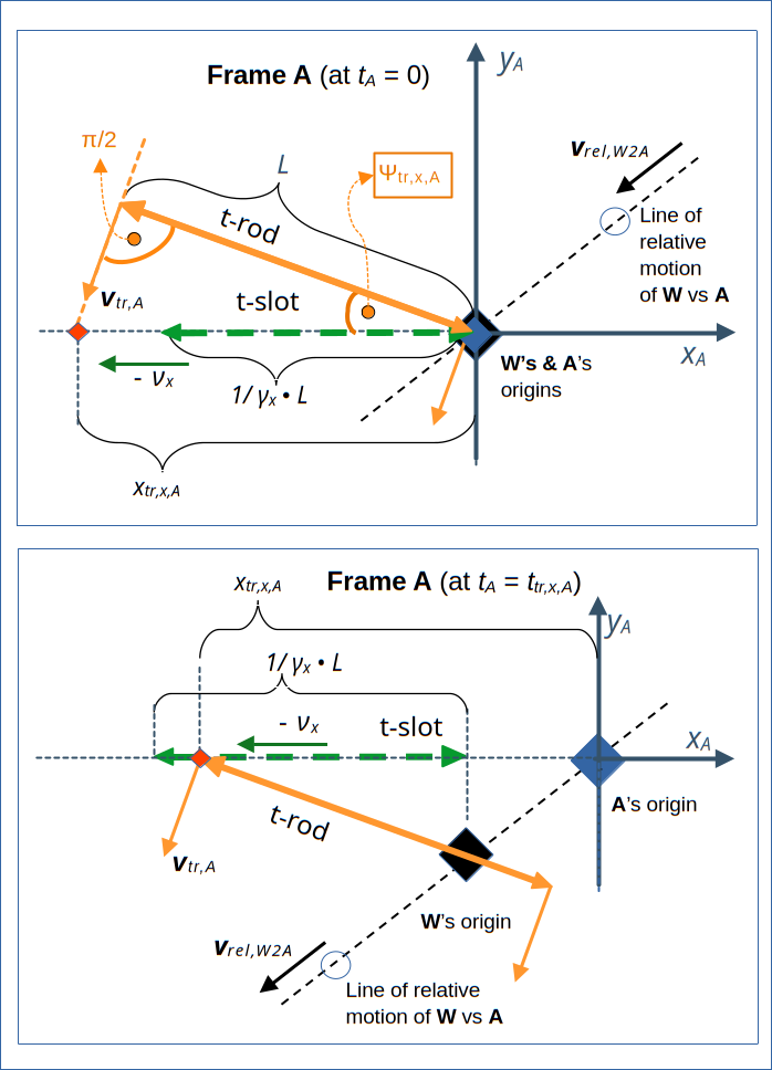
Development of the transit scenario in setup frame A for the collision scenario

Illustration 2: Schematic representation of the development of the transformed transit scenario from the perspective of an observer attached to frame A. Although the t-slot is perceived to have a shorter length than the t-rod, the velocities and the timing are such that the t-rod gets through the t-slot’s extension. The start of the transit starts under somewhat extreme conditions, which are due to our initial conditions for the transit scenario in W.

If our two conditions are fulfilled a logical analogy consideration shows that the transit will be possible for any point on the t-rod between 0 ≤ t_A ≤ t_tr,x,A for our given constant velocities.

The upper drawing in illustration 2 shows that the point where the t-rod’s left end touches the x_A-axis has a coordinate X_tr,x,A given by

\[ X_{tr,x,A} \,=\, – \, {1 \over |\cos \left( \Psi_{tr,x,A} \right)| }\, L \, =\, \gamma_x\, N^{1/2} \,L \,. \]

A short calculation shows that the time t_tr,x,A is given by the distance, which the t-rod’s left end has to overcome, divided by its velocity v_tr,A

\[ t_{tr,x,A} \,=\, X_{tr,x,A} * \sin\left( \Psi_{tr,x,A} \right) * {1 \over v_{tr,A}} \,. \]

Using relations from above, this results in

\[ t_{tr,x,A} \,=\, \gamma_x \, \beta_x \, N^{1/2} * {L \over c} \,. \]

Now, let us look at the x-coordinate X_ts,L,A for the t-slot’s left end at t_A = t_tr,x,A :

\[ \begin{align} X_{ts,L,A} \,&=\, – \left[ \, {1 \over \gamma_x}\, L \, + \nu_x * t_{tr,x,A} \, \right], \\[8pt] &=\, – \, L \, \left[ \, {1 \over \gamma_x} \,+\, \gamma_x \, \beta_x^2 \, N^{1/2} \, \right] \,. \end{align} \]

The difference of the absolute values of our positions is given by :

\[ \begin{align} |X_{ts,L,A}| \, – |x_{tr,xA}| \,& =\, L \, \left[ \, {1 \over \gamma_x} \,+\, \gamma_x \, \beta_x^2 \, N^{1/2} \,-\, \gamma_x \,N^{1/2} \, \right] \\[8pt] &= \, {1 \over \gamma_x}\, L * \left[\, 1 \,-\, N^{1/2} \,\right] \,\, \Rightarrow \\[10pt] |X_{ts,L,A}| \, – |x_{tr,xA}| \,&\gt\, 0\,, \,\, \mbox{as} \,\, N \,<\, 1 \,. \end{align} \]

And for the respective right end of the t-slot we get a coordinate X_ts,R,A and a respective difference of

\[ \begin{align} |x_{tr,xA}| \,-\, |X_{ts,R,A}| \,& =\, L \, \left[ \, \gamma_x \,N^{1/2} \,-\, \gamma_x \, \beta_x^2 \, N^{1/2} \, \right] \\[8pt] &= \, \gamma_x \, N^{1/2}\, L * \left[\, 1 \,-\, \beta_x^2\,\right] \,\, \Rightarrow \\[10pt] |x_{tr,xA}| \,-\, |X_{ts,R,A}| \,&\gt\, 0 \,. \end{align} \]

This is exactly what we need for a transit of the t-rod through the t-slot from the perspective of an observer attached to frame A! We have just shown that the transit scenario also works from the perspective of an observer in A. Yeah, of course, we can trust in the Lorentz Transformation!

Side remark: As we have seen already in previous posts, the event, when the left end passes the slot, happens at a later point in time than when the t-rod’s right end passes the slot. In W these two events happen at the same time, namely t_W = 0. This is nothing unusual. Events that are perceived to happen at the same time in a certain reference frame, may happen at different times in another. We have seen this already multiple times when we applied the LT both to the collision and the transition scenario to derive the perception of observers moving with the objects.

The tangent of the differences in the velocity components between the t-rod and the origin of W

We now prove a very useful relation which will help us to interpret the transit scenario at times t_A < 0. We look at the differences of the velocity components of the t-rod in y_A– and x_A-direction vs. respective velocity components of the origin of W. The velocity components of the origin of W and the respective inclination angle Ψ_WA of its path in A are given by:

\[ \begin{align} v_{x, W2A} \, = \, -\, \beta_x * c \,, \quad v_{y, W2A} \,=\, – \,\beta_y * c \,. \\[10pt] \cos \left( \Psi_{WA} \right) \,= \, {\beta_x \over \beta_{rel}}\,, \quad \sin \left( \Psi_{WA} \right) \,=\, {\beta_y \over \beta_{rel}} \,. \\[10pt] \end{align} \]

See post XIII for more details about a diagonal moving frame W. Note that we have defined the angle Ψ_WA as a positive one for the inclination between the x_A-axis and the line of relative motion between the frames W and A.

Now, the absolute values of the velocity differences Δv_w,tr,x,A and Δv_w,tr,y,A between the origin of W and the t-rod the along the x_A-axis and the y_A-axis, respectively, are:

\[ \begin{align} |\Delta v_{w,tr,x,A} | \,&=\, | v_{x, W2A} \,-\, v_{tr,x,A} | \\[8pt] &=\, c\, \beta_x * \left[ \,1 \,-\, {1\over N}\, \gamma_x^2\, \beta_y^2 \, \right] \\[8pt] &=\, {1 \over N} \, {1 \over \gamma_{rel}^2} \, \beta_x \, c \,, \\[10pt] |\Delta v_{w,tr,y,A} | \,&=\, | v_{y, W2A} \,-\, v_{tr,y,A} | \\[8pt] &=\, c\, \beta_y * \left[ \,1 \,-\, {1\over N} \, \right] \\[8pt] &=\, {1 \over N} \, {1 \over \gamma_{rel}^2} \, \gamma_x^2 \, \beta_x^2 \, \beta_y \, c \,. \end{align} \]

Hence,

\[ { |\Delta v_{w,tr,x,A} | \over |\Delta v_{w,tr,y,A} | } \,=\, \gamma_x^2\, \beta_x\, \beta_y \,= \, \tan\left( \Psi_{tr,x,A} \right) \,. \]

This links the movements of the t-rod and the origin of W strongly in A; see the illustrations below.

Direct comparison of the collision and the transit scenario in frame A

We have proven that the transit of the rod through the slot, which we cleverly defined in W, remains a transit in A, too. Our settings provided us with two fully equivalent slots in A and even the lengths of the t-rod and the c-rod are equal there. So, we are well prepared for a direct comparison of the conditions for our two scenarios in our standard frame A.

I firstly show a direct comparison at t_A = 0:

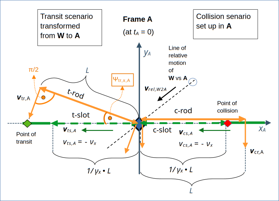
Direct comparison of a transit scenario with a collision scenario for equivalent slots

Illustration 3: A direct comparison of the standard collision scenario with a (transformed) transit scenario in frame A. The acute inclination angle of the t-rod vs. the t-slot enables a transit of the longer t-rod through the t-slot. In the collision scenario, however, the c-rod will inevitably collide with a plate to the right of the c-slot. This demonstrates that transit and collision scenarios with parallelly moving and otherwise equivalent slots require very different setup conditions.

In the drawing above I have indicated the plates to the left of the t-slot and to the right of the c-slot.

We clearly see that if we want to get a working transit scenario for a t-slot, which is fully equivalent to the c-slot of the collision scenario, and for a t-rod with the same length L as the c-rod, we need initial conditions with an acute inclination angle Ψ_tr,x,A between the t-rod and the t-slot.

This is actually something, which we found already intuitively in post VIII and which we confirmed in posts IX to XI about the transit scenario. Of course, we also need a subtle setting of the ratios between the velocity components of the rod and the slot’s horizontal velocity.

Note once again: The essential point in this comparison is the choice of completely equivalent slots; they have the same perceived length and velocity in both scenarios. Even the rods have identical lengths. For a different type of comparison see the next post.

We get it that the presentation of the rod/slot paradox as discussed in the very first post of this series has an essential deficit and argues based on an error:

A comparison of observer perceptions based on describing the perspective of observers attached to objects, which move in two dimensions, must not disregard inclination angles enforced by a proper use of the Lorentz Transformation. Which in turn results in the Thomas-Wigner rotation of diagonally moving objects.

Hopefully, my readers have become more and more aware of this simple truth during this post series.

Now, let us go a bit backward to a point in time t_A < 0 with our comparison. Then we get something like this :

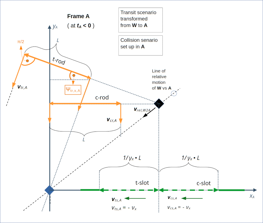
Illustration 4: A direct comparison of the collision scenario with a transit scenario in frame A – at a time t_A < 0, i.e. some time before the encounter. The strong coupling of the movement of the t-rod with the motion of W in A is a result of the relation of the velocity of the t-rod in W with the frames’ relative motion there.

The depicted relation between the orientation and position of the t-rod with the origin of W is due to the specific choice of velocity components in W and the resulting relations for relevant angles in A.

The bottom line of our comparison is:

A transit scenario requires specific settings in the very same frame used set up a natural collision scenario – and vice versa. These settings must reflect the Thomas-Wigner rotation of elongated objects moving diagonally in an observer’s frame. A simple change of perspectives as in the standard presentation of the rod/slot paradox without taking care of this relativistic rotation effect is simply wrong and incompatible with the Lorentz Transformation.

Conclusion

All conflicts which the rod/slot paradox seemingly, but wrongly implies are caused by a wrong assumption of what different observers would perceive for the rod/slot encounter and/or related initial conditions.

Changing the perspective of an observer residing in a standard setup frame for either scenario to the perspective of an observer co-moving with one of the objects must take care of the impact of the Thomas-Wigner rotation on the other object. This rotation results from a proper use of the Lorentz Transformation in two dimensions. This relativistic effect leads to inclination angles, which are disregarded in the standard presentation of the rod/slot paradox.

The Thomas-Wigner rotation causes inclination angles of either the rod or the slot or both vs. each other and vs. naturally chosen x-axes after the Lorentz Transformations between different reference frames. These inclinations actually save the consistency of the scenario descriptions across different reference frames and in particular between observers attached to the moving rod/slot objects.

A direct comparison of a working transit scenario with a collision scenario for equivalent slots and for rods of equal lengths in one and the same frame illustrates the resulting (and required) differences in the initial conditions in a striking manner.

In the next and concluding post of this series I will give you some hints regarding the non-commutativity of a sequence of two Lorentz Transformations along non-collinear axes. We will investigate what this actually means for a change from our standard setup frame A to a diagonally frame W via a sequence of two LTs.

Stay tuned …