Special relativity and the rod/slot paradox – XIV – angle between colliding rod and slot in a diagonally moving frame

I continue my post series on the 2-dimensional rod/slot paradox in Special Relativity. In this post we perform a Lorentz Transformation of the rod from a frame A, which we previously used to describe a collision scenario, to a diagonally approaching frame W. W is related to a frame Z used for the setup of the transit scenario (see below). In a previous post we have already derived results for the transformed slot coordinates in W. A comparison will show that there is a constant angle between the rod and the slot in W.

Proper coordinates of the rod’s right end for a transformation between frames A and W

I remind you of the conditions in frame A at a time ahead of the rod/slot encounter in the collision scenario. The encounter happens at t_A = 0. The drawing below shows the relative movement of reference frame W vs. frame A. The origins of the frames coincide at t_A = t_W = 0. At this point in time also the left ends of the rod and the slot meet.

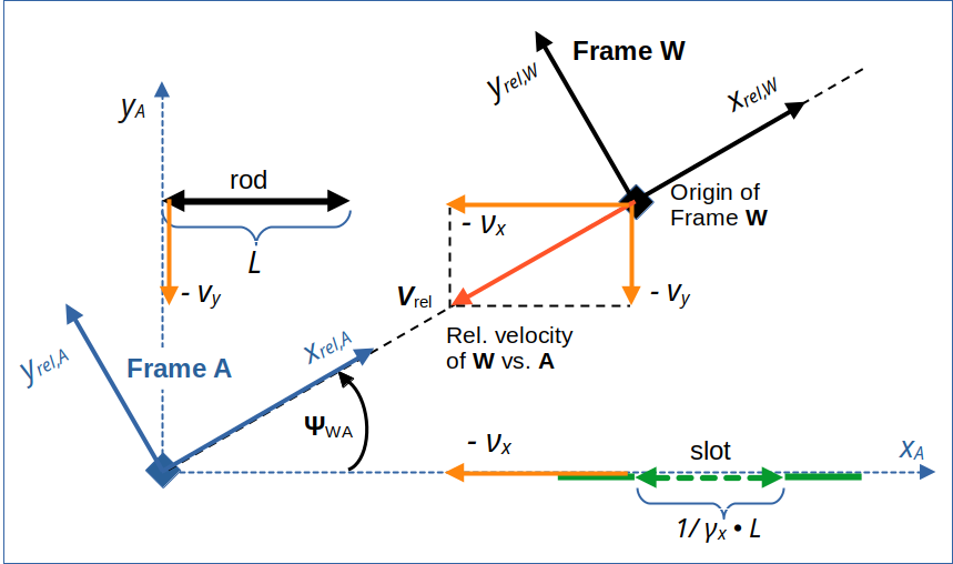
Rotated coordinate systems of frames A and W

Illustration 1: A diagonally approaching frame W in our collision scenario, which set up in a frame A. For a Lorentz Transformation from A to W we use rotated Cartesian coordinate systems with x-axes oriented along the line of relative motion of the frames.

For details, certain quantities, abbreviations and terminology see previous posts.

At time t_A = t_W = 0 it is relatively easy to find out how the rod is oriented in W – with respect to the line of relative motion between A vs. W. Analogously to the steps in the previous 13th post we first calculate components of the position vectors for the rod’s left end right end at t_A = 0 with respect to the line of relative motion. The component x_r,r,rel,A of the position vector to the rod’s right end parallel to the line of relative motion is

\[ x_{r,r,rel,A}(t_A=0) \,=\, L * \cos \left(\Psi_{WA} \right) \, =\, L\,{\beta_x \over \beta_{rel}} \,. \]

But for the LT to W we have to use a different event to ensure that the respective time coordinate in A is transformed to t_W = 0. The velocity components v_r,x,rel,A of the the rod parallel to the relative line of motion and the respective vertical component v_r,y,rel,A are

\[ \begin{align} v_{r,x,rel,A} \,&=\, -\, v_y * \sin \left( \Psi_{WA} \right) \, =\, -\, v_y \, {\beta_y \over \beta_{rel}} \,, \\[8pt] v_{r,y,rel,A} \,&=\, -\, v_y * \cos \left( \Psi_{WA} \right) \, =\, -\, v_y \, {\beta_x \over \beta_{rel}} \,. \end{align} \]

From the LT of time coordinates between A and W we derive that we need an event at a point in time

\[ t_{r,r,rel,A} \,=\, -\,{v_{rel} \over c^2 } \, x_{r,r,rel,A}(t_A=t_{r,r,rel,A}) \,. \]

Due to the motion of the right end of the rod we have

\[ x_{r,r,rel,A}(t_A=t_{r,r,rel,A}) \,= \, L*\cos\left(\Psi_{WA}\right) \,+\, v_{r,x,rel,A} * t_{r,r,rel,A} \,. \]

This leads to

\[ t_{r,r,rel,A} \,=\, -\, {v_{rel} \over c^2} \, \left[ \, L \,{\beta_x \over \beta_{rel} } \,-\, v_y \, {\beta_y \over \beta_{rel} } \, t_{r,r,rel,A} \,\right] \,. \]

Which resolves after some intermediate steps to

\[ t_{r,r,rel,A} \,=\, – {1 \over c} \, \beta_x \, \gamma_y^2 \, L \,. \]

In turn we get the required x_r,r,rel,A-coordinate at t_A = t_r,r,rel,A :

\[ t_A = t_{r,r,rel,A} \,: \quad x_{r,r,rel,A} \,=\, \gamma_y^2 \, {\beta_x \over \beta_{rel} } \, L \,. \]

The respective vertical component of the position vector is

\[ \begin{align} t_A = t_{r,r,rel,A} \,: \quad y_{r,r,rel,A} \,&=\, – L \,\sin \left( \Psi_{WA} \right) \,+\ v_{r,y,rel,A} * t_{r,r,rel,A} \\[8pt] &= \, {\beta_y \over \beta_{rel} } \, L \,+\, v_y \,{\beta_x \over \beta_{rel}} *{1 \over c} \, \beta_x \, \gamma_y^2 \, L \,, \end{align}\]

which after some steps gives

\[ t_A = t_{r,r,rel,A} \,: \quad y_{r,r,rel,A} \,=\, – \, {\beta_y \over \beta_{rel} } \, {\gamma_y^2 \over \gamma_{rel}^2 } \, L \,. \]

Transformation of rod’s coordinates at t_A = t_W = 0 to frame W

The spatial coordinates of the left end of the rod transform to W simply as

\[ t_W = 0\,: \quad x_{r,l,rel,W} \,= 0, \quad y_{r,l,rel,W}\,=\, 0 \,. \]

Note that in W we also work with a (rotated) coordinate system that has an x-axis (x_rel,W) aligned with the line of relative motion of A vs. W. The LT for the spatial coordinates of the right end of the rod tells us

\[\begin{align} x_{r,r,rel,W} \,&=\, \gamma_{rel} \,\left[\, \gamma_y^2 \, {\beta_x \over \beta_{rel} } \, L \,+\, v_{rel} \, \left( -\, {1 \over c} \right) \beta_x\,\gamma_y^2 \,L\,\right] \\[8pt] &=\, \gamma_{rel} \,\gamma_y^2 \, \beta_x \,L \, \left[ \,{1 \over \beta_{rel}} \,-\, \beta_{rel} \,\right] \,. \end{align}\]

After some intermediate steps we find

\[\begin{align} x_{r,r,rel,W} \,&=\, {\gamma_y^2 \over \gamma_{rel}} \, {\beta_x \over \beta_{rel} } \, L \,, \\[8pt] y_{r,r,rel,W} &=\, – \, {\gamma_y^2 \over \gamma_{rel}^2 } \, {\beta_y \over \beta_{rel} } \, L \,, \\[8pt] t_{r,r,rel,W} &=\, 0 \,. \end{align}\]

Length of the rod in W

The length of the rod in W becomes

\[\begin{align} L_{rod,W}^2 \,&=\, x_{r,r,rel,W}^2 \,+\, y_{r,r,rel,W}^2 \\[8pt] &=\, – \, {\gamma_y^2 \over \gamma_{rel}^2 } \, {\gamma_y^2 \over \gamma_{rel}^2 } \, {1 \over \beta_{rel}^2 } \, L^2 * \left[ \, \beta_x^2 \, \gamma_{rel}^2 \, +\, \beta_y^2\,\right] \,. \end{align}\]

This gives results in

\[\begin{align} L_{rod,W}^2 \,&=\, {\gamma_y^2 \over \gamma_{rel}^2 } \, L^2 \quad \Rightarrow \\[8pt] L_{rod,W} \,&=\, {\gamma_y\over \gamma_{rel} }\, L \,\lt\, L \,. \end{align}\]

Orientation of the rod in W with respect to the line of relative motion

By using results from the previous posts we get for the angle between the rod and the line of relative motion in W

\[ \begin{align} \cos \left( \Psi_{r,rel,W} \right) \,&=\, { x_{r,r,rel,W} \over L_{rod,W}} \, =\, \gamma_y \,{\beta_x \over \beta_{rel}} \\[8pt] &=\, \gamma_y \, {\gamma_{rel} \over \gamma_x} * \cos \left( \Psi_{s,rel,W} \right) \, \Rightarrow \\[8pt] \cos \left( \Psi_{r,rel,W} \right) \,&\gt \cos \left( \Psi_{s,rel,W} \right) \,. \end{align} \]

This means

\[ 0 \,\lt\, \Psi_{r,rel,W} \,\lt\, \Psi_{s,rel,W} \,. \]

The rod is smaller than L in W, but there is an angle between the slot and the rod !

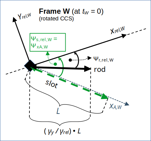
Illustration 2: Rod and slot at t_W = 0 in frame W. x_rel,W and y_rel,W are the coordinate axes of a coordinate system with x-axis aligned with the line of relative motion of A vs. W.

So, seen from the slot the situation is very similar to what we previously found for the collision scenario in frame B. But we have to get an idea about the velocities of the rod and the slot before we understand the resulting kinematics.

Conclusion

The collision scenario as seen from a diagonally approaching frame appears to be similar to what an observer in frame B sees. There is an angle between the slot and the rod. In the next post we want to check whether the velocities in W guarantee a collision.