Special relativity and the rod/slot paradox – VII – no paradox for a collision scenario and consistency between all relevant LTs

In the previous posts of this series I have shown that the so called “rod/slot paradox” may disappear for a well defined collision scenario. We have taken the perspectives of observers in different reference frames and applied the Lorentz Transformation [LT] to selected key events. So far, we have found different, but consistent descriptions of the predefined rod-slot collision. In this post we conclude the analysis of our collision scenario by performing a transformation from a frame C co-moving with the rod to a frame B co-moving with the slot. We will again find a clear prediction of a collision – consistent both with the description of observers in a setup frame A and previous Lorentz Transformations from A to frames B and C and from frame B to C.

This last LT is in so far relevant as the initial conditions in frame C completely pre-define the collision. In the end we can therefore forget about our special setup frame A and instead focus on the perceptions of observers attached to the physical objects in relative diagonal motion versus each other. Special Relativity transforms a parallel orientation of the rod and the slot in the rod’s frame to an inclination angle between rod and slot in the slot’s frame. And this rotation effect guarantees consistency regarding the prediction of a collision.

Collision scenario, previous key results and objectives

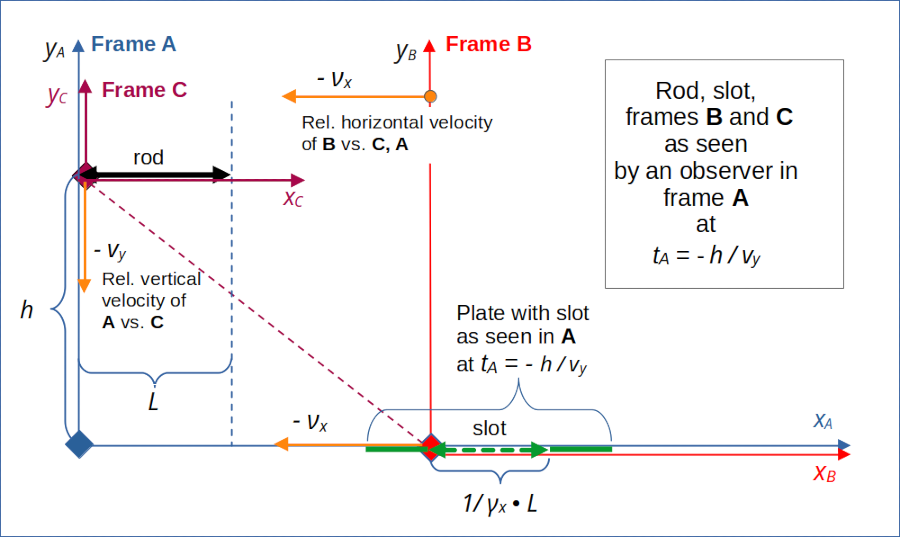
For the setup of our collision scenario and notations for kinematic quantities see posts I to III. Our collision scenario was defined in a frame A, in which the rod and the slot were oriented parallel to the x_A-axis and moved with constant velocities along the y_A-axis and the x_A-axis, respectively. See the following drawing:

rod, slot, frames B and C as seen from frame A

Illustration 1: Setup of the collision scenario as seen in frame A. The relative diagonal motion of the rod versus the slot in the chosen spatial coordinate systems ensures that the left ends of the rod and slot meet at collision time t_A = t_B = 0. Length contraction affects the slot and ensures a collision of the rod with an assumed plate around the slot. The dotted line illustrates the relative motion of the rod and the slot schematically.

We have already checked the consistency of the results of Lorentz transformations [LTs] between some of the different reference frames. This included frames attached to our physical objects, namely the rod (frame C) and the slot (frame B). We calculated key event data by applying LTs leading from frame A to frame B (co-moving with the slot) and to frame C (co-moving with the rod), respectively. In post VI we have in addition proved the consistency of all data by a direct LT between frames B and C based on the relative velocity of the rod vs. the slot.

Previous results and inclination angles

We first used standard Cartesian coordinate systems for the frames B and C, such that the respective x-axes were aligned with the rod and the slot, respectively. I.e. the slot (and its surrounding plate) stretched along the x_B-axis and the rod lay on the x_C-axis. See the drawings. With respect to these coordinate systems the rod and the slot approached each other via a diagonal movement in two dimensions. We have found that the inclination of the relative line of motion with the rod as perceived in frame C differed from the inclination with the slot as measured in frame B.

After the application of a LT from A to B we saw that the rod was not only moving diagonally vs. the slot, but that it also showed an inclination angle vs. the slot and the x_B-axis. We also derived that an observer in frame C would measure the inclination angle between the rod and the slot to be zero. We confirmed this by the application of LTs of event coordinates first from A to C, from A to B and later on from B to C.

By the LT from B to C we started to really focus on relativity – without leaning on the somewhat artificial setup frame A. In the end all that matters are the physical objects, their relative motion and the measurements of related observers. We took the key event coordinates as measured by a B-observer moving with the slot as given and transformed them to a frame attached to the rod.

Mathematically the last step got a bit complicated – as we could not apply a full relativistic vector formalism in four-dimensional space-time, but used our familiar and the most simple (basically 1-dimensional) form of the LT along the vector of the rod’s relative motion v_rel,CB as seen in frame B.

Perception of colliding rod's movement by the slot

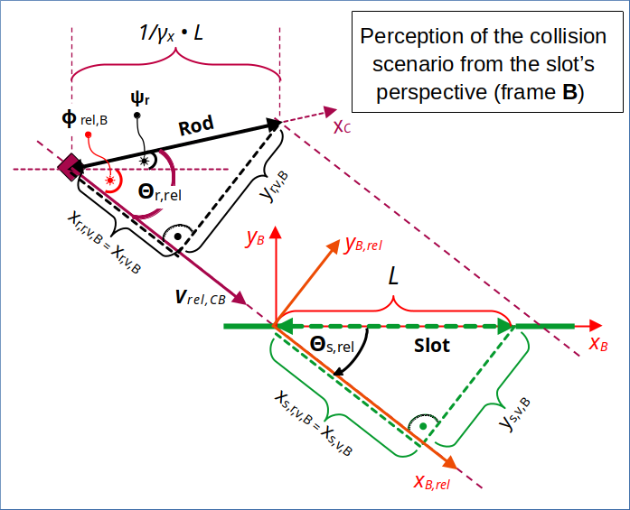
Illustration 2: The moving rod as perceived by observers in a frame B attached to the slot. The slot is at rest in frame B. The x_B-axis of a B-related standard coordinate coordinate system is aligned with the slot. A rotated coordinate system instead has an x_B,rel – axis aligned with the vector of the rod’s relative diagonal velocity v_rel,CB towards the slot (as seen from the slot’s perspective!).

Note the inclination angle Ψr of the moving rod vs. the slot in frame B. For details see the 3rd and the 4th posts of this series.

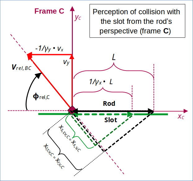
Well, from the rod’s perspective (i.e. from observers in frame C) things look a bit different – as we have already shown by previous (independent) calculations:

Illustration 3: Collision of diagonally moving slot with rod as seen from the rod’s perspective (frame C). I have indicated projections of the slot and rod onto the line given by the vector of the slot’s relative velocity v_rel,BC to the rod. The rod is at rest in frame C.

Note that we have shown in post V that

\[ \Psi_{rel,C} \ne \Psi_{rel,B} \,. \]

Objective of this post

We will apply a Lorentz transformation to event coordinates given in frame C and derive respective coordinates in frame B. As displayed above, the conditions in frame C clearly indicate a collision. By independent calculations done in the first posts of this series we have already derived results for an inclination angle between rod and slot in frame B. This inclination guaranteed the collision of the rod with the plate around the slot in frame B. Our objective is to show that a direct LT using the relative velocity v_rel,BCbetween the slot and the rod (as seen in C) reproduces these results.

A consistent result would mean that observers moving along with the physical objects agree upon the physical consequences of the initial conditions perceived by them. This step completes our proof of consistent predictions concerning the rod/slot collision by all relevant frames of reference. We use “ECS” as an abbreviation for a Cartesian coordinate system (in a flat Euclidean space).

The steps to be performed are analogous to the ones in 4th post of this series:

Determine the components of the relative velocity vector of the slot in the rod’s frame C and its respective angle Φ_rel,C with the x_C-axis.
Turn to a rotated ECS with an x-axis (x_C,rel – axis) aligned with the relative velocity vector v_rel,BC.
Perform projections of position vectors to points on the rod and the slot onto the relative velocity vector to get components parallel and perpendicular to the line of relative motion. This corresponds to finding spatial event coordinates for the rod’s and the slot’s right ends in the rotated ECS.
Apply the standard Lorentz Transformation to the event-coordinates in the rotated ECS (with a gamma-factor derived from the absolute value of the relative velocity of the the slot vs. the rod).
Re-transform the resulting coordinates (parallel and perpendicular to the relative velocity vector) in frame B to coordinates in the standard ECS of B (whose x_B-coordinate axis is aligned with the slot).

We will use some formulas already established in previous posts.

Transformation of coordinates of selected events at the rod’s end points

We know already (see post V) that the angle of the relative velocity vector with the x_C-axis in frame C is given by:

\[ \cos \left(|\Phi_{rel,C}| \right) = {1 \over \gamma_y} \, {\nu_x \over v_{rel} }, \quad \sin \left(|\Phi_ {rel,C}|\right) = {v_y\over v_{rel} } \, , \]

with

\[ \begin{align} \pmb{\operatorname{C}} : & \pmb{v}_{rel,BC} = \pmb{v}_{rod,C} \, = \, \left( \, – {1 \over \gamma_y} \nu_x, \,\, \, v_y \, \right) \,, \\[8pt] & v_{rel} = | \pmb{v}_{rel,CB} | = | \pmb{v}_{rel,BC} | = \left[ \, {1 \over \gamma_x^2} \, v_y^2 \, + \, \nu_x^2 \, \right]^{1/2} \,, \\[8pt] & \quad \quad = \left[\, {1 \over \gamma_y^2}\, \nu_x^2 \,+\, v_y^2 \, \right]^{1/2} \,, \\[8pt] & \gamma_{rel} = \left[1 – {v_{rel}^2 \over c^2} \right]^{-1/2} \, = \, \gamma_x * \gamma_y \,\,. \end{align} \]

For a position vector from the origin to the slot’s right end we get the following component data x_r,v,C (parallel to the line of relative motion) and y_r,v,C (perpendicular to the line of relative motion) in the rotated ECS:

Rod’s vector components parallel and perpendicular to relative velocity vector

\[ \begin{align} x_{r,v,C} \,&=\, { 1\over \gamma_y} \,{\nu_x \over v_{rel}} * L \,, \\[10pt] y_{r,v,C} \,&=\, {v_y \over v_{rel}} * L \,. \end{align} \]

Event selection

When selecting events – and in particular respective time coordinates – we have to be careful to choose events whose transformation gives us a resulting identical time coordinate in frame B. The reason is that an observer in frame B is naturally interested in the positions of the rod’s ends at the same point in time. We choose the target time coordinate to be t_B = 0 (collision time):

\[ t_B = 0 \,. \]

Let us call the x-, y-, t-coordinates of events for the left and the right ends of the rod in the rotated coordinate systems of frames C and B

x_r,l,v,C , y_r,l,v,B , t_r,l,v,B and x_r,r,v,C , y_r,r,v,C , t_r,r,v,C
and
x_r,l,v,B , y_r,l,v,B , t_r,l,v,Band x_r,r,v,B , y_r,r,v,B , t_r,r,v,B ,

respectively.

We pick the following events for the left end of the rod (E^v_r,l) and the right end of the rod (E^v_r,r) in frame C to get respective spatial coordinates in frame B at t_B = 0:

\[ \begin{align} \mbox{Rod’s left end :} \quad &\pmb{\operatorname{E}}_{r,l}^v \sim \left [\, x_{r,l,v,C},\,\, y_{r,l,v,C},\,\, t_{r,l,v,C} ,\right ]_C \\[8pt] & = \left [\, 0,\,\, 0,\,\, 0\,\right ]_C , \\[10pt] \mbox{Rod’s right end :} \quad &\pmb{\operatorname{E}}_{r,r}^v \sim \left [\, x_{r,r,v,C},\,\, y_{r,r,v,C},\,\, t_{r,r,v,C} ,\right ]_C \\[8pt] &= \left [\, x_{r,v,C},\,\,\, y_{r,v,C}, \,\,\, – v_{rel}/c^2 * x_{r,v,C} \,\right ]_C \,. \end{align} \]

Application of the Lorentz Transformation to the selected coordinates of the rod’s ends

Application of the Lorentz transformation (along the line of motion and relative velocity v_rel ) gives us:

\[ \begin{align} x_{r,r,v,B} \,&=\, \gamma_x * \gamma_y * \left[ \, x_{r,r,v,C} \,+\, v_{rel} \, {(-v_{rel}) \over c^2} * x_{r,r,v,C} \,\right] \\[8pt] &= \, \gamma_x * \gamma_y * \left[ \, x_{r,v,C} \,- \, { v_{rel}^2 \over c^2} * x_{r,v,C} \,\right] \\[8pt] &= \gamma_x* \gamma_y * \left( 1 \,-\, {v_{rel}^2 \over c^2} \right) * x_{r,v,C} \,=\, {1 \over \gamma_x * \gamma_y} * x_{r,v,C}\\[8pt] &= \, {1 \over \gamma_x * \gamma_y ^2} \, { \nu_x \over v_{rel} } * L \,, \\[10pt] y_{r,r,v,B} \,&=\, y_{r,v,C} \,= \, {v_y \over v_{rel}} * L \,, \\[10pt] t_{r,r,v,C} \,&=\, \gamma_x * \gamma_y * \left[ {-v_{rel} \over c^2} * x_{r,v,C} \,+\, {v_{rel} \over c^2} * x_{r,v,C} \right] = 0 \, . \end{align} \]

The transformation for the rod’s left end gives us:

\[ x_{r,l,v,B} \,=\, 0, \quad y_{r,l,v,B} \,=\, 0, \quad t_{r,l,v,B} \,=\, 0 \,. \]

The reader may compare this to the respective coordinates for our selected events found in a previous post (using results of a LT from frame A to frame B). They data are identical with what we independently got above !

The rest is a simple geometrical back-transformation from the rotated spatial coordinate system in B to the standard coordinate system there (with its x_B-axis aligned with the slot). I leave this to the reader.

Just, to be on the safe side, let us check for the length of the rod in frame B – as given by the transformed data:

\[ \begin{align} L_{rod,B}^2 \,&=\, \left[\, {1 \over \gamma_x^2 * \gamma_y^2} \, {1 \over \gamma_y^2} \, {\nu_x^2 \over v_{rel}^2} \,+\, { v_y^2 \over v_{rel}^2} \,\right] * L^2 \\[8pt] & =\, \left[\, {1 \over \gamma_{rel}^2} \, \left( 1- \beta_y^2\right) \, {\nu_x^2 \over v_{rel}^2 } \,+\, { v_y^2 \over v_{rel}^2} \, \right] * L^2 \\[8pt] & =\, \left[\, \left(1 – { v_{rel} \over c^2} \right) \, \left( 1- \beta_y^2\right) \, {\nu_x^2 \over v_{rel}^2 } \,+\, { v_y^2 \over v_{rel}^2} \, \right] * L^2 \\[8pt] & =\, \left[\, { v_y^2 \over v_{rel}^2} \,+\, {\nu_x^2 \over v_{rel}^2 } \,-\, {\nu_x^2 \over c^2} \,-\, \beta_y^2\, { \nu_x^2 \over v_{rel}^2} \,+\, \beta_x^2* \beta_y^2 \, \right] * L^2 \\[8pt] & =\, \left[\, { v_y^2 \over v_{rel}^2} \,+\, {\nu_x^2 \over v_{rel}^2 } \,-\, {\nu_x^2 \over c^2} \,-\, \beta_y^2\, { \nu_x^2 \over v_{rel}^2} \,+\, \beta_x^2* \beta_y^2 \, \right] * L^2 \\[8pt] & =\, \left[\, { v_y^2 \over v_{rel}^2} \,+\, {\nu_x^2 \over v_{rel}^2 }\, \left( 1 – \beta_y^2\right) \,-\, \beta_x^2 \,+\, \beta_x^2* \beta_y^2 \, \right] * L^2 \\[8pt] & =\, \left[\, { 1 \over v_{rel}^2} \, \left(v_y^2 \,+\, {\nu_x^2 \over \gamma_y^2 } \right) \,-\, \beta_x^2 \,+\, \beta_x^2* \beta_y^2 \, \right] * L^2 \\[8pt] & =\, \left[\, 1 – \beta_x^2 \,+\, \beta_x^2* \beta_y^2 \, \right] * L^2 \\[8pt] & =\, \left[\, {1 \over \gamma_x^2} \,+\, \beta_x^2* \beta_y^2 \, \right] * L^2 \,. \end{align} \]

This means

\[ L_{rod,B} = L * \left[ \, 1 \,-\, \beta_x^2 \, \left(1 – \beta_y^2 \right) \,\right]^{1/2} \, \lt L \,. \]

This is exactly what we independently found in the 4th post of this series.

With some trigonometry you can also derive the angles Θ_r,rel and Ψ_r (see illustration 1):

\[ \begin{align} \cos \left(|\Psi_r |\right) \, &=\, \cos \left( |\Theta_{r,rel,B} – \Phi_{rel,B} \right) \\[8pt] &=\, \cos \left( |\Theta_{r,rel,B} |\right) * \cos \left( |\Phi_{rel,B}| \right) \,+\, \sin \left(|\Theta_{r,rel,B}|\right) * \sin \left(|\Phi_{rel,B} |\right) \\[8pt] &=\, {1 \over \gamma_x * \gamma_y} \, {1 \over \gamma_y } \, {\nu_x \over v_{rel}} \, {L \over L_{rod,B} } * {\nu_x \over v_{rel}} \,+\, {v_y \over v_ {rel}} \, {L \over L_{rod.B}} * {1 \over \gamma_x}\, {v_y \over v_{rel}} \\[8pt] &=\, {1\over \gamma_x} \,{1\over v_{rel}^2} \,{\nu_x^2 \over \gamma_y^2} \, {L \over L_{rod,B} } \,+\, {1 \over \gamma_x} \,{v_y^2\over v_{rel}^2} \, {L \over L_{rod,B} } \\[8pt] &=\, {1 \over \gamma_x} \,{L \over L_{rod,B}} \,. \end{align}\]

This is exactly, what we have independently found this in 5th post. It also means:

\[ x_{r,r,B} \,=\, L_{rod,B} * cos\left(|\Psi_r|\right) = {1 \over \gamma_x} * L \,, \]

which, of course, is correct and consistent with what we derived in the 4th post by a LT from A to B.

Application of the Lorentz Transformation to coordinates of the slot

Let us look at the slot. Here we expect that a LT from frame C to frame B reproduces

\[ L_{slot,B} \,=\, L \,, \quad \mbox{and} \quad \Psi_{s,B} \,=\, 0 \,, \]

with Ψ_s,B meaning the angle between the slot and the x_B-axis.

Before applying the LT, please remember that the slot is a moving object in frame C. In contrast to the rod, we therefore have to consider the special position x_s,v,c of the slot in the rotated coordinate system at a special time t_s,v,C which transforms to t_B = 0. The conditions by the LT for the right end of the slot are:

\[ \begin{align} \mbox{LT : } &\quad t_{s,r,v,B} \,= \, \gamma_{rel} * \left[\, t_{s,v,C} \,+\, {1 \over v_{rel}^2} \, x_{s,v,C} \, \right] = 0 \\[8pt] &\Rightarrow \quad t_{s,v,C} \,=\, – {v_{rel} \over c^2} \, x_{s,v,C} \\[10pt] \mbox{rod motion : } &\quad x_{s,v,C} \,=\, x_{s,r,v,C} – v_{rel} * \left( – {v_{rel} \over c^2} \, x_{s,v,C} \right) \,, \\[8pt] &\Rightarrow \quad x_{s,v,C} \,=\, \left( 1 – {v_{rel}^2 \over c^2} \right)^{-1} * x_{s,r,v,C} \,. \\[8pt] &\Rightarrow \quad x_{s,v,C} \,=\, \gamma_{rel}^2 * x_{s,r,v,C} \,. \end{align} \]

In addition we have (see posts V and VI):

\[ \begin{align} x_{s,r,v,C} \,&=\, {1 \over \gamma_x }\,L * \cos\left (|\Phi_{rel,C}|\right) \\[8pt] &=\, {1\over \gamma_x}\,L * {1 \over \gamma_y} \,{\nu_x \over v_{rel}} \,, \\[10pt] y_{s,r,v,C} \,&=\, \, {1 \over \gamma_x }\,L * \sin \left (|\Phi_{rel,C}|\right) \\[8pt] &=\, {1\over \gamma_x}\,L * {v_y \over v_{rel}} \,. \end{align} \]

Putting these special data into the into the LT along the line of relative motion gives us:

\[ \begin{align} x_{s,r,v,B} \, &= \, \gamma_{rel} * L * \left[\, x_{s,v,C} \, – \, { v_{rel}^2 \over c^2} \, x_{s,v,C} \,\right] \\[8pt] &= \, \gamma_{rel} * x_{s,v,C} * \left( 1 – { v_{rel}^2 \over c^2 } \right) \\[8pt] &= \, {1 \over \gamma_{rel}} * \gamma_{rel}^2 * {1 \over \gamma_{rel}} \, {\nu_x \over v_{rel}} \, L \\[8pt] & = \, {\nu_x \over v_{rel}} * L \, \\[10pt] y_{s,r,v,B} \,&=\, y_{s,r,v,C} \,=\, {1\over \gamma_x} \, {v_y \over v_{rel}} * L \,, \\[10pt] t_{s,r,v,B} &= 0 \,. \end{align} \]

Hence

\[ \begin{align} L_{slot,B}^2 \,&=\, x_{s,r,v.B}^2 \,+\, y_{s,r,v,B}^2 \\[8pt] &=\, {1 \over v_{rel}^2} * L^2 * \left[\, \nu_x^2 \,+\, \left({v_y\over \gamma_x}\right)^2 \,\right] \\[8pt] &=\, L^2 \,. \end{align} \]

Furthermore, we get for the inclination angle Θ_s,rel of the slot with the line of the rod’s relative motion in B:

\[ \begin{align} \cos \left( |\Theta_{s,rel}|\right) \, &= \, {x_{s,r,v,B} \over L } \, =\, {\nu_x \over v_{rel}} \\[8pt] &= \, \cos \left(|\Phi_{rel,B} |\right) \,. \end{align}\]

Which means that the angle Ψ_s,B between the slot and the x_B-axis according to the LT from C to B indeed is found to be zero:

\[ \Psi_{s,B} = 0 \,. \]

This shows that a direct Lorentz transformation from frame C to B, i.e. between observers co-moving with the rod and the slot, respectively, reproduces the results which we got by a transformation from our setup frame A to the slot’s frame B.

Conclusion

We have studied a carefully prepared collision scenario with a rod that diagonally approaches a slot, and with both the rod and the slot having the same proper length. The length contraction effect clearly forced an observer in the setup frame to predict a collision. By using Lorentz transformations, we have shown that observers in all relevant frames

the setup frame A,
a frame B attached to the slot
and a frame C attached to the rod

would predict a collision of the rod with a plate around the slot. The various Lorentz Transformations between the different frames did not produce any contradiction. Hence the paradox does not exist for our standard collision scenario. Observers in different frames have different perceptions regarding details of the scenario as e.g. inclination angles of the rod vs. the slot or concerning the relative velocity vs. the frame’s x-axis. However, they all agree on an inevitable collision.

The paradox obviously had its origin in a wrong description of the initial conditions in the slot’s frame: The usual standard description simply ignores inclination angles predicted by the Lorentz Transformation.

Now, after all of our complex considerations, there are still open questions:

Is there a scenario in which the rod may pass the slot unharmed? And would such a “transit scenario” lead to some strange contradiction with our collision scenario?

This is the topic of some forthcoming posts as e.g.

Special relativity and the rod/slot paradox – VIII – setup of a transit scenario with the rod moving through the slot

Stay tuned ….