Can the universe be infinite? – III – basic solutions of the Friedmann equation

In the first post of this series we have picked up the question whether a Big Bang at the beginning of the universe and a finite speed of light imply a finite universe. In the 2nd post we saw that the assumption of a time dependent scaling factor for all distances between objects, which passively co-move with a cosmic fluid, is compatible with the cosmological principle [CP]. Based on Newtonian physics we came up with the so called first and second Friedmann equations for an evolving universe.

In this post we derive the usual three solutions of the Friedmann equation. There are ore, we will come back to, later. The math involves some integrals which have to be evaluated. The way of integration is a bit different in the literature. For those interested, I present a direct way (also used of R. & H Sexl in a introductory book [1]), but also two equivalent and more elegant ways. The latter approaches provide some additional insights in a proper choice of coordinates.

Those readers who are not so much interested in solving integrals may directly go to the plots below and think a bit about the questions posed in a respective section.

Previous posts:

Repetition: Friedmann equations

Let me remind you of the structure the Friedmann equations (based on Newtonian considerations). The 1st Friedmann equation is

\[ \ddot{a}(t) \, = \, -\, {4 \over 3}\, \pi \, G\, \rho_0 * a(t) \, , \tag{1} \]

and the 2nd Friedmann equation looks like

\[ \left( {\dot{a} \over a} \right)^2 \, = \, {8 \, \pi \, G \over 3 } \, \rho(t) \, – \ { k \over a^2} \, , \tag{2} \]

k came into the game as an integration constant. We had rewritten eq. (2) as

\[ \begin{align} &\dot{a}^2(t) \, – \, {C \over a(t)} + k \,=\, 0 \, , \tag{3} \\[8pt] \quad &\mbox{with} \,\,\, C \,=\, {8 \over 3}\, \pi \, G\, \rho_0 \, a_0 \,. \end{align} \]

As da/dt covers a scaled expansion and thus dr/dt of distant objects, k reflects some combined energy in the Newtonian picture. Note the following aspects:

Any violation of the homogeneity or isotropy assumptions of the cosmological principle would induce modifications of the equations.
So far we have not specified what the “density” ρ(t) may include. We need an idea of contributing parts as matter, radiation and other stranger components. I will later come back to this question in later posts – as it may affect the structure of solutions.
We have not assumed any shear or viscous forces affecting matter flow. The matter in our model universe behaves as if t were an ideal fluid. For the time being we assume non-relativistic, viscuous-free dust-like matter. (But we keep in mind that radiation may contribute to the gravitational potential.)
So far we have not assumed some separate cosmological constant (representing some kind of vacuum energy).
(- k) can be interpreted as a kind of “total energy” – as the first term in (3) reminds of a kinetic energy and the second of some potential (gravitational) energy.
In the Newtonian picture the total mass mass could be finite – without changing the basic equations which led to the Friedmann equations. For consequences of a limited total mass of the universe, see a question in the final section.

Preparation of direct integration

To get a clear view about what eq. (3) implies for a development of a(t), we need to integrate. By a variable separation we see

\[ dt \,=\, \pm {da’ \over \sqrt{ C / a’ \,- \, k} } \,. \tag{4} \]

We know that a(t) ≥ 0. Let us in addition assume a(t=0) = 0. This means that the universe started an expansion at t = t_BB = 0. We get to the integral equations

\[ \begin{align} t \,- \, t_{BB} \,=\, t \,&=\, \int_0^{a(t)} { { 1 \over \sqrt{ C / a’ \,- \, k} } \, d{a’} } \,, \tag{5} \\[8pt] t_S \,-\, t \,&=\, \int_0^{a(t)} { { 1 \over \sqrt{ C / a’ \,- \, k} } \, d{a’} } \,. \tag{6} \end{align} \]

The solution range depends heavily on k and the sign of da/dt. We call the integral F(a(t)):

\[ F(a(t)) \,:=\,\int_0^{a(t)} { { 1 \over \sqrt{ C / a’ \,- \, k} } \, d{a’} } \,. \tag{7} \]

From (4) we see

\[ \begin{align} \dot{a} \,\ge\, 0 \, : \quad & t \,= \, F (a(t))\,, \tag{8} \\[6pt] \quad &\mbox{for } k \le 0 \,\,\mbox{or} \,\, \left( k \gt 0 \land C/a \ge k \right)\,, \\[10pt] \dot{a} \,\lt \, 0 \, : \quad & t’ \,=\, t_S\, -\, t \,= \, F (a(t))\,, \tag{9} \\[6pt] \quad &\mbox{with } k \gt 0 \land C/a \ge k \,. \end{align} \]

t_S has yet to be determined. We also have to watch the impact of C/a -> k,at the upper integral border. The integral itself depends strongly on “k“. We have to distinguish at least 3 possibilities:

(1) k > 0, (2) k = 0, (3) k < 0.

The first case makes life a bit hard.

Symmetric solution for k > 0

Equ. (3) tells us that da/dt can become zero and thus reach a maximum. Equ. (3) also tells us something about the symmetry of the solution: For each value of a(t) we have two solutions of da/dt – a positive one and a negative one of equal size:

\[ \begin{align} a(t_+) = a(t_-) = A \, : \quad \Rightarrow \quad \dot{a}(t_+) \,&= \, +\, \sqrt{ {C \over A}^{\phantom{2}} – \,k} \, , \\[10pt] \dot{a}(t_{-}) \,&= \, -\, \sqrt{ {C \over A}^{\phantom{2}} – \, k} \,. \end{align} \tag{10}\]

\[ \dot{a}^2(t) \,=\, 0, \quad \mbox{for} \,\, {a(t) \over C } \,=\, {1 \over k} \,. \]

Another point is that the derivative gets infinitely big for small a:

\[ a(t) \rightarrow 0 \,\,\Rightarrow \,\, \dot{a}(t) \rightarrow \infty \,. \]

Why is the symmetry important? Because of the maximum of a(t) at some time t_max we are not able to get the full solution from the integral (7) alone. Instead we may have to use symmetry considerations and obey eq. (9) in the regime of a declining a(t).

Integration for k > 0

The integration is a bit tricky. Therefore, I show some intermediate steps. First we note that

\[ {d \over da’} \left({C \over a’}\right) \,=\, -\, C {1 \over {a’}^2} \,\Rightarrow\, da’ \,= \, – {a'{^2} \over C } * d \left({C\over a’}\right)\,. \]

Therefore, with a new variable u = C/a’ > k we can rewrite our integral (7)

\[ F_+ \,=\, F(k\gt 0) \,=\, C \, \int_{C/a(t)}^{\infty} { {1\over u^2 \, \sqrt{u-k} } \,du} \,. \tag{11} \]

Looking this up in integral tables gives us

\[ \begin{align} F_+ \,&=\, {C \over k} \, \left[ {\sqrt{\left(v-k\right) } \over v} \,+\, {1\over 2}\, {2 \over \sqrt{k}} \arctan\left( { 1 \over \sqrt{k} }\, \sqrt{v – k} \right) \right]_{C/a(t)}^{\infty} \\[10pt] &=\, {C \over k} \, \left[ {1 \over \sqrt{k}} \, \pi/2 \,-\, \sqrt{\ {a\over C} \,-\, k\, \left( {a\over C} \right)^{2^{\phantom{2}}} } \,-\, {1 \over \sqrt{k}} \, \arctan\left( {1 \over \sqrt{k}} \, \sqrt{ {C \over a}^{\phantom{2}} – k \,} \, \right) \right] \,. \end{align} \]

We first rewrite the argument to the arctan:

\[ \begin{align} &\arctan\left( {1 \over \sqrt{k}} \, \sqrt{ {C \over a}^{\phantom{2}} – k \,} \, \right) \\[10pt] =\,\, &\arctan \left( {1 \over \sqrt{ {k\, a \over C} } } \, \left[ \, 1 \,-\, \left( \sqrt{ {k\, a \over C} } \,\right)^2 \,\right]^{1/2} \, \right) \,. \end{align} \]

With this argument the arctan can be transformed into an arccos (see the Internet for inverse trigonometric functions):

\[ F_+ =\, {C \over k} \, \left[ {1 \over \sqrt{k}} \, \pi/2 \,-\, \sqrt{\ {a\over C} \,-\, k\, \left( {a\over C} \right)^{2^{\phantom{2}}} } \,-\, {1 \over \sqrt{k}} \, \arccos\left( \sqrt{ {k\, a \over C} } \right) \right] \, . \]

The arccos can further be be changed :

\[ F_+ \, =\, {C \over k} \, \left[ {1 \over 2 \, \sqrt{k}} \, \left( \pi \,-\, \, \arccos\left( {2\, k\, a \over C} \,-\, 1 \right) \right) \,-\, {1 \over \, \sqrt{k}} \, \sqrt{\ {k\, a\over C} \,-\, \left( {k\, a\over C} \right)^{2^{\phantom{2}}} } \,\, \right] \,, \]

and thus

\[ F_+ \, =\, {C \over k} \, {1 \over \sqrt{k}} \, \left[ {1 \over 2 } \, \arccos\left( 1 \,-\, 2\, {k\, a \over C} \right) \,-\, \sqrt{ {ka\over C} \,-\, \, \left( {k\, a\over C} \right)^{2^{\phantom{2}} } } \,. \right] \tag{12} \]

For a somewhat more clever way of integrating see below. We recognize that we can only evaluate this expression for

\[ 0 \,\le \, {k \, a \over \, C} \,\le \, 1 \,. \]

This gives us an upper limit of a(t) as the upper border of our integral. When a(t) reaches a maximum a_max value this happens at a time t_ma :

\[ a_{max} = {C \over k} \,\quad \Rightarrow \,\quad t_{ma} = { C \over k } \, {1 \over \sqrt{k}} \,{\pi \over 2} \,. \]

So, at t_ma, we reach some kind of maximum extension of this type of model universe. In the sense that the scale parameter reaches a maximum everywhere . I.e. distances between objects co-moving with the expanding cosmic “fluid/dust” reach a maximum with da/dt(t_ma) = 0.

Extension to t > π/2 : It is clear that the artificial border of our integral evaluation does not prevent a prolongation of a proper solution to values t > t_ma . Before using a coordinate transformation to get rid of the integrals limitations, let us use some (somewhat sloppy) symmetry arguments:

We have not yet looked at the negative integration of (6) and (9). The respective solution must fulfill the condition the derivative of a takes a negative sign (but the same absolute value) at other locations t’ with the same value of a(t). A solution which just mirrors a(t) with respect to t_me fulfills this condition – and has both a(t_ma) and da/dt(t_ma) in common with its mirrored original part. From this we may assume that

\[t_S \,=\, {C \over k^{3/2} } \,\pi \,. \]

The arccos also allows for a different solution. The question is how we can use this option to create a proper symmetric solution. To make things a bit easier let us focus on the case k = +1. Let us furthermore introduce t_c = t/C and a_c = a/C. A symmetric solution is then given if we assume
a_c(π – t) = a_c(t) plus t_c‘ = π – t_c.

\[ t’_c = \pi – t_c \, \land\, a_c(t’_c) = a_c(t_c) \, , \,\, \, k\,=+1 \,. \]

The negative solution (9) tells us for k = +1 :

\[ t’_c \, =\, t_S \,-\, t_c \,, \quad \mbox{with} \,\, a_c(t’_c) = a_c(t_c) \,. \]

At t_c= π/2 we actually have t_S= 2 t_c

\[ t_c \,=\, \pi / 2 \,: \quad t_S \, – \, t_c \, = \, t_c \,\Rightarrow \,\, t_S = \pi \,. \]

Do we get something similar via the variability of arccos-values? According to eq. (12) the expression for t_c has the structure

\[ t_c \,=\, {1 \over 2} \, \Gamma_{acos} \,-\, \Gamma_{sqr} \,, \quad ( k \,=\, +1) \,.\]

We get the same result when we use arccos(x) = arcos(x-2π) – which throws the result in a negative region. We write

\[ t_c” \, = – t_c’ \,=\, \, -\,\pi \,+\, {1 \over 2} \, \Gamma_{acos} \,-\, \Gamma_{sqr} \, = \, -\,\pi + t_c \,,\]

as we want the alternative solution t_c‘ to be positive. This gives us again

\[ t_c’ \,=\, \pi \, -\, t_c \,, \quad \mbox{for} \,\, a_c(t’_c) = a_c(t_c) \,. \]

So, we are on the right track here for a continuous continuation fulfilling our derivative condition. In the general case we find or alternative time value to be

\[ t’ \,=\, {C \over k^{3/2} } \,\pi \, -\, t \,, \quad \mbox{with} \,\, a(t’) = a(t) \,. \]

Integration for k < 0

The result for k < 0 given in the introductory book of Sexl [1] is unfortunately wrong. I therefore give a derivation here. We use K = -k and start with

\[ F_- \,=\, F(k \lt 0) \,=\, C \, \int_{C/a(t)}^{\infty} { {1\over u^2 \, \sqrt{u+K} } \,du} \,, \quad K = -k \,. \tag{10} \]

We find a solution in an integral table. This gives us after an evaluation of the different terms for the border values a square root and an inverse hyperbolic function. Sorry, but it simply is that complicated. Plots below will later later to understand the solution behavior .

\[ F_- \,=\, {C \over K} \left[ \sqrt { {a\over C} + K\, \left({a\over C}\right)^{2^{\phantom{2}}} \, } \,-\, {1 \over \sqrt{K}} \operatorname {arccoth} \left( {1 \over \sqrt{K}} \, \sqrt{ {C \over a} + K } \right) \, \right] \,. \tag{11} \]

By using arctanh(x) = arccoth(1/x) this can again be transformed to

\[ F_- \,=\, {C \over K} \left[ \sqrt { {a\over C} + K\, \left({a\over C}\right)^{2^{\phantom{2}}} \, } \,-\, {1 \over \sqrt{K}} \operatorname {arctanh} \left( { \sqrt{K\, a/C} \over \sqrt{ 1 + \left(\sqrt{K\, a/C}\right)^2 } }\, \right) \, \right] \,. \tag{12} \]

By using a relation with the arcsinh we arrive at

\[ F_- \,=\, {C \over K} \left[ \sqrt { {a\over C} + K\, \left({a\over C}\right)^{2^{\phantom{2}}} \, } \,-\, {1 \over \sqrt{K}} \operatorname {arcsinh} \left( \sqrt{K\, {a\over C} } \, \right) \, \right] \,. \tag{13} \]

Integration for k = 0

Simple, just look up the integral.

Three standard solutions

After this exhausting effort, we obviously have to distinguish three formal “solutions”:

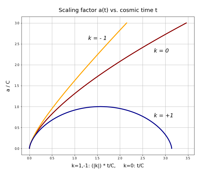
\[ \begin{align} k\,\gt\, 0\,\, &: \quad {k^{3/2} \,t \over C} \,=\, {1 \over 2 } \, \arccos \left(\,1 \,-\, 2 \, {k\, a \over C} \, \right) \,-\, \sqrt{ {k\, a \over C}\,-\, \left({k\, a\over C}\right)^{2^{\phantom{1}} } } \,, \\[8pt] &\quad\quad \mbox{for} \,\, {k^{3/2} \,t \over C} \le \pi/2 \quad \mbox{and mirrored for } \,\, \pi/2\,\lt \, { k^{3/2} \,t \over C} \le \pi \,,\\[10pt] k \,=\, 0\,\, &: \quad {t \over C} \,=\, {2 \over 3} \, \left({a \over C} \, \right) ^{3/2} \,, \\[10pt] k \,\lt\, 0\,\, &: \quad {|k|^{3/2}\,t \over C} \,=\, \sqrt{ {|k| \, a \over C}\,+\, \left( {|k| \,a\over C} \right)^2 \, } \,-\, \, \operatorname {arcsinh} \left( \sqrt{{|k|\, a\over C} } \, \right) \,\,. \end{align} \]

Now, you may miss an explicit representation in the functional form a(t) = f(t) . However, we can numerically calculate t(a) and invert it. For k > 0 we evaluate the integral only to a maximum possible value of a(t) – and afterward use symmetric mirroring with respect to t_ma.

The following plots show results for k = 1, k = 0, k = -1:

Better ways of integrating

An experience one has to get used to in some corners of theoretical physics is that coordinate transformations may help to deal with integrals and their borders. Our objective is to come to a more compact presentation covering the full spectrum of possible values for t and a variables – also for k > 0.

Without loosing much generality for our discussion, we focus on the case k = +1. We again use the scaled variables t_c and a_c :

\[ k\,=\, + 1\,, \quad a_c \,=\, {a \over C}\,, \quad t_c \,=\, {t \over C} \,. \]

The maximum value of a_c = 1. Our differentials can be rewritten as

\[ dt_c \,=\, \pm \, {da_c’ \over \sqrt{ 1 / a_c’ \,- \, 1} } \,=\, \pm \, {\sqrt{ a_c’} \, da_c’ \over \sqrt{1 \,-\, a_c’} } \]

Integration via substitution with an angle for a/a_max

Looking at the graphical solution, the symmetry reminds us of trigonometric functions. We could get into this regime by interpreting a_c‘ as the square of a kind of “cosmic” angle” φ_c, i.e.

\[ a_c’ \,=\, \sin^2 \phi_c \,. \]

We integrate and get

\[ \begin{align} t_c \, &=\, + \, {\large \int}_0^{\phi_c} \, { \sqrt{ \sin^2 \phi_c } \over \sqrt{ \cos^2 \left( \phi_c \right)^{\phantom{1}} } } \, 2 \, \sin (\phi)\, \cos (\phi) \, d\phi \,, \quad 0 \le \phi \le \pi/2 \,, \\[8pt] t_c \, &=\, – \, {\large \int}_{\phi_c}^{\pi} \, { \sqrt{ \sin^2 \phi_c } \over \sqrt{ \cos^2 \left( \phi_c \right)^{\phantom{1}} } } \, 2 \, \sin (\phi)\, \cos (\phi) \, d\phi \,, \quad \pi/2 \le \phi \,. \end{align} \]

Regarding the borders: We used the maximum range of the angle with a_c‘ varying from 0 to 1 and back to 0. The plus sign in front of the integral corresponds to da/dt > 0, i.e. . When resolving the square root of the cos we need to use the minus sign for π/2 < φ_c ≤ π. This cancels then against the (- cos) in the upper part. Thus, the integrand in both integrals becomes the same – and we can simplify to

\[ \begin{align} t_c \, &=\, \int_0^{\phi} \, 2 \, \sin^2 \phi \, d\phi \, = \, \int_0^{\phi} \, [ 1 \, – \cos (2 \phi)] \, d\phi \\[8pt] &= \, \phi_c – {1 \over 2}\, \sin 2 \phi_c \,. \end{align} \]

We introduce a new variable η via setting 2φ = η and end up with

\[ \begin{align} 0 \le \eta \le \pi \,: \quad t_c \,&=\, {1 \over 2}\, \left( \eta \,-\, \sin \eta \right) \,, \\[8pt] a_c \,&=\, {1 \over 2}\, \left( 1 \,-\, \cos \eta \right) \,. \end{align} \]

We have arrived at a concise presentation form, but with a dependence on a new variable. It would be nice to get some physical interpretation of η. See below.

Integration via “conformal time”

A look into a table of integrals reveals: The integral over a square root becomes relatively simple when we have a quadratic term of the integration variable under the square root. To get such a term we would have to multiply the square root with a. Let us focus again on the cases k = +1. We introduce a new variable ξ by setting

\[ \begin{align} &d \xi \,=\ {1 \over a_c(t) }\, dt_c\,, \\[8pt] &\Rightarrow \,\, \xi \,-\, \xi_0 \,=\, \int_0^{t_c} \, {1\over a_c'(t_c’)} \, dt_c’ \,, \\[8pt] &\Rightarrow \,\, \xi \,-\, \xi_0 \,=\, \int_0^{a_c(t_c)}\, {1 \over \sqrt{ a_c’\,-\, \,{a’_c}^2} } \, da_c’ \tag{20} \,, \\[8pt] &\Rightarrow \,\, t_c \,-\, t_{c_0} \,=\, \int_0^{\xi} \, a_c(\xi)\, d\xi \,. \tag{21} \end{align} \]

With ξ₀ = 0, the integral over a_c‘ can be resolved :

\[ \begin{align} \xi \,&=\, {\pi \over 2 } \, – \, \arcsin \left( 1 \, -\, 2\, a_c\right) \\[8pt] 2 a_c \, -\, 1 \,&=\, \sin( \xi \,-\, \pi/2 ) \,. \end{align} \]

Using trigonometry this gives us

\[ \begin{align} a_c \, &= \, {1 \over 2} \, ( 1 \,-\, \cos \, \xi) \,, \\[8pt] t_c \, &= \, {1 \over 2} \, ( \xi \,-\, \sin \, \xi)\,. \end{align} \]

Comparing with the results we got above we find

\[ \xi = \eta \quad \Rightarrow \quad d\eta \, = \, {dt \over a_c} \,. \]

η is called the “conformal time“.

Without going into details we can apply the substitution also for the case k = -1. Our basic integral then has a different logarithmic solution, which can be mapped to the inverse of the hyperbolic cosine cosh. Using respective transformation formulas we eventually get:

\[ \begin{align} k\,=\ + 1\,\, &: \quad {t \over C } \,=\, {1 \over 2}\, \left( \eta \,-\, \sin \eta \right) \,, \\[8pt] &\quad\quad {a \over C } \,=\, {1 \over 2}\, \left( 1 \,-\, \cos \eta \right) \,, \quad \eta \gt 0 \,, \\[10 pt] k \,=\, 0\,\, &: \quad {t \over C} \,=\, {2 \over 3} \, \left({a \over C} \, \right) ^{3/2} \,, \quad \quad \quad t \gt 0 \,, \\[10pt] k \,=\, -1 \,\, &: \quad {t \over C} \,=\, {1 \over 2}\, \left( \sinh \eta \,- \, \eta \right) \,, \\[8pt] &\quad\quad {a \over C } \,=\, {1 \over 2}\, \left( \cosh \eta \,-\, 1 \right) \,, \quad \eta \gt 0 \,. \\[10 pt] \end{align} \]

I leave it to the reader to include k into the formulas. We at least have found a rather consistent form for the different cases. We can use this for further discussions. Plotting the a(t) with the above formulas gives us the same result as shown above.

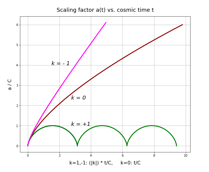
However, with the help of the conformal time we can now extend the solution to bigger t-values, also for positive values of k:

A first interpretation

Some important points of the above solutions of the Friedmann equations are the following:

k > 0 opens space for a cyclic evolution of the scaling factor of distances. For k ≤ 0 we must assume that the distances between observers and objects in the cosmic fluid/dust will grow forever.
The solutions tell us that there was a kind of beginning in the sense that the cosmic scaling started at a respective time coordinate t = t_c = ξ = 0. For k > 0, we could regard this as an intermediate point in a cyclic evolution. However, for k ≤ 0 we must assume an original beginning of the universe in the past.
The parameter k scales the evolution in time and in space – and couples respective coordinates. Its constant everywhere and can be regarded as a fundamental property of the universe. As said, we momentarily have no clue what that might mean.
At t = t_c = ξ = 0 the different k-dependent developments of the scaling factor a(t) converge. So the conditions at the beginning of the scaling of distances in our model are almost the same.

We call the beginning of the scaling the “Big Bang“. The questions below do, however, indicate that we do not understand how such a beginning could start at all. The plots above indicate that [(da/dt) / a] gets smaller with time for all cases. We call

\[ H(t) \,=\, {\dot{a}(t) \over a(t)} \]

the “conformal Hubble expansion factor“. Obviously, it is not a constant of time. For our present time t = t₀

\[ H(t_0) \,=\, {\dot{a}(t_0) \over a(t_0)} \]

it is called the “Hubble constant“.

We have assumed a dust like behavior of the matter which is conserved inside defined and scaled regions. Therefore, the matter/energy density also scales in a defined way. However, other components in the real universe, as relativistic photons, may scale differently with matter density. This will have an impact on the solution of the Friedmann equation.

Questions to the reader

(1) The constant k came into the game as an integration constant. A physical interpretation should be given, too. In the Newtonian picture: Which meaning could k have?
(2) We have assumed a(t=0) = 0. What kind of observation in our real universe would support this view? Theoretically: What would have changed in our line of argumentation if we had assumed a contracting universe?
(3) The Friedmann equations imply a dynamic universe. The behavior of a depends on both time and k. And distances for k ≤ 0 would increase forever. In the Newtonian interpretation (da/dt) / a(t) at a given point in time means that dr/dt ∝ r (see the previous post).
Does that mean that galaxies moving radially away from us reach flight velocities larger than the speed of light? But not for an observer closer to the receding objects? Is the Friedmann equation therefore not compatible with special relativity? If the Friedmann equation were true – and all observers experience the cosmic scaling in the same way: Can any coordinate system attached to any observer be interpreted as an inertial system, at all? If so, in what sense?
(4) The time dependence of the scaling factor for all k indicates that for t -> 0 the distances between objects in our cosmic dust went to zero a(t) -> 0, for t -> 0. We saw that this view holds for any observer.
Does this imply that our universe was finite at t=0?
(4a) When distances to our neighboring galaxies in the cosmic fluid were smaller and smaller at t -> 0: Would an observer not have seen more and more matter/galaxies in his surroundings in the early universe?
(4b) Take a given amount of matter around an observer. Let us move back in time to t -> 0: Then matter would contract systematically – and (ignoring effects of an equation of state) at some point in time concentrate inside a respective Schwarzschild radius. Would that not mean that the universe had to exist fragmented in black holes everywhere at some time close to the Big Bang? Or in reverse: How could the universe have come into existence at all – if nothing can leave a black hole?
(5) Given the assumptions we put into the Newtonian derivation of the Friedmann equations and assuming that we observe galaxies moving away from us according to the described dynamics: Would our results not be compatible with a picture assuming that we indeed sit at the center of the universe and that all matter is finite and arranged in concentric shells with equal mass density around us up to a maximum distance? That would imply a real edge of the universe.
(5a) What parts of the cosmological principle would such a picture contradict?
(5b) By what kind of observations could we prove such a (crazy) configuration? Consider different cases for the total amount of mass and the described dynamics.
(5c) Assume that our coordinate system is indeed a preferred one and that we either have reflecting or open boundary conditions at the universe’s edge for radiation. What would other observers see? What would either boundary condition mean for an assumed photon gas in the universe?
(6) In a cyclic universe for k > 0 : What about the 2nd law of thermodynamics?

Criticism of Newtonian assumptions

If you try to answer some of the questions posed below, you may find that we are in trouble regarding the definition of an adequate coordinate system to describe the assumed expansion. Either we must assume that we are in a very special position in the universe. Or we have problems finding a coordinate system marking an absolute space, because with the dynamic solution above everything seems to move against all other things. The uniform scaling of distances indicates a new kind of relativity. In consistency with the CP, the scaling factor has the same effects everywhere – each and every observer sees all other objects in the cosmic fluid receding from his/her position.

The whole situation is as if a (potentially infinite) space creates more space between otherwise not moving objects. This does not seem to fit the Newtonian picture of an ever equal and static space. We found an equation, but we have extreme difficulties to interpret its message in a static invariable space.

In the next post we will give the Friedmann equations another basement. Stay tuned …

Literature / Links

[1] Roman u. Hannelore Sexl, 1979, “Weiße Zwerge, schwarze Löcher”, Verlag Friedr. Vieweg und Sohn, Braunschweig